Category Archives: Temperature History

Can’t Be Explained by Natural Causes

The fact that CO2 in the atmosphere can cause warming is fairly settled.  The question is, how much?  Is CO2 the leading driver of warming over the past century, or just an also-ran?

Increasingly, scientists justify the contention that CO2 was the primary driver of warming since 1950 by saying that they have attempted to model the warming of the last 50 years and they simply cannot explain the warming without CO2.

This has always struck me as an incredibly lame argument, as it implies that the models are an accurate representation of nature, which they likely are not.  We know that significant natural effects, such as the PDO and AMO are not well modelled or even considered at all in these models.

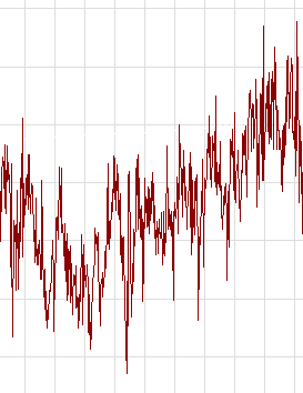
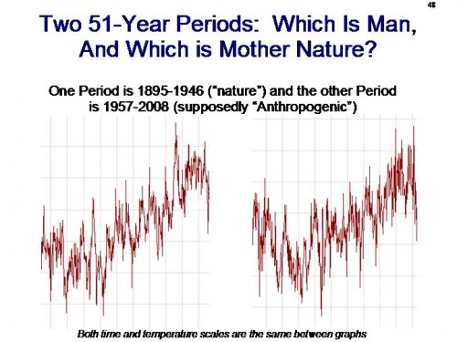
But for fun, lets attack the problem in a different way.  Below are two global temperature charts.  Both have the same scale, with time on the X-axis and temperature anomaly on the Y.   One is for the period from 1957-2008, what I will call the “anthropogenic” period because scientists claim that its slope can only be explained by anthropogenic factors.  The other is from 1895-1946, where CO2 emissions were low and whose behavior must almost certainly be driven by “nature” rather than man.

Sure, I am just a crazy denier, but they look really similar to me.  Why is it that one slope is explainable by natural factors but the other is not?  Especially since the sun in the later period was more active than it was in the earlier “natural” period.  So, which is which?

slide48

Continue reading Can’t Be Explained by Natural Causes

Regression Abuse

As I write this, I realize I go a long time without getting to climate.  Stick with me, there is an important climate point.

The process goes by a number of names, but multi-variate regression is a mathematical technique (really only made practical by computer processing power) of determining a numerical relationship between one output variable and one or more other input variables.

Regression is absolutely blind to the real world — it only knows numbers.  What do I mean by this?  Take the famous example of Washington Redskins football and presidential elections:

For nearly three quarters of a century, the Redskins have successfully predicted the outcome of each and every presidential election. It all began in 1933 when the Boston Braves changed their name to the Redskins, and since that time, the result of the team’s final home game before the election has always correctly picked who will lead the nation for the next four years.

And the formula is simple. If the Redskins win, the incumbent wins. If the Redskins lose, the challenger takes office.

Plug all of this into a regression and it would show a direct, predictive correlation between Redskins football and Presidential winners, with a high degree of certainty.  But we denizens of the real world would know that this is insane.  A meaningless coincidence with absolutely no predictive power.

You won’t often find me whipping out nuggets from my time at the Harvard Business School, because I have not always found a lot of that program to be relevant to my day-to-day business experience.  But one thing I do remember is my managerial economics teacher hammering us over and over with one caveat to regression analysis:

Don’t use regression analysis to go on fishing expeditions.  Include only the variables you have real-world evidence really affect the output variable to which you are regressing.

Let’s say one wanted to model the historic behavior of Exxon stock.  One approach would be to plug in a thousand or so variables that we could find in economics data bases and crank the model up and just see what comes out.  This is a fishing expedition.  With that many variables, by the math, you are almost bound to get a good fit (one characteristic of regressions is that adding an additional variable, no matter how irrelevant, always improves the fit).   And the odds are high you will end up with relationships to variables that look strong but are only coincidental, like the Redskins and elections.

Instead, I was taught to be thoughtful.  Interest rates, oil prices, gold prices, and value of the dollar are all sensible inputs to Exxon stock price.  But at this point my professor would have a further caveat.  He would say that one needs to have an expectation of the sign of the relationship.  In other words, I should have a theory in advance not just that oil prices affect Exxon stock price, but whether we expect higher oil prices to increase or decrease Exxon stock price.   In this he was echoing my freshman physics professor, who used to always say in the lab — if you are uncertain about the sign of a relationship, then you don’t really understand the process at all.

So lets say we ran the Exxon stock price model expecting higher oil prices to increase Exxon stock price, and our regression result actually showed the opposite, a strong relationship but with the opposite sign – higher oil prices seem to correlate better with lower Exxon stock price.  So do we just accept this finding?  Do we go out and bet a fortune on it tomorrow?  I sure wouldn’t.

No, what we do instead is take this as sign that we don’t know enough and need to research more.  Maybe my initial assumption was right, but my data is corrupt.  Maybe I was right about the relationship, but in the study period some other more powerful variable was dominating  (example – oil prices might have increased during the 1929 stock market crash, but all the oil company stocks were going down for other reasons).  It might be there is no relation between oil prices and Exxon stock prices.  Or it might be I was wrong, that in fact Exxon is dominated by refining and marketing rather than oil production and actually is worse off with higher oil prices.    But all of this points to needed research – I am not going to write an article immediately after my regression results pop out and say “New Study: Exxon stock prices vary inversely with oil prices” without doing more work to study what is going on.

Which brings us to climate (finally!) and temperature proxies.  We obviously did not have accurate thermometers measuring temperature in the year 1200, but we would still like to know something about temperatures.  One way to do this is to look at certain physical phenomenon, particularly natural processes that result in some sort of annual layers, and try to infer things from these layers.  Tree rings are the most common example – tree ring widths can be related to temperature and precipitation and other climate variables, so that by measuring tree ring widths (each of which can be matched to a specific year) we can infer things about climate in past years.

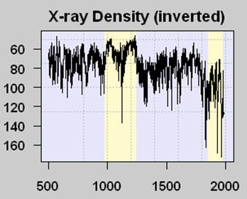
There are problems with tree rings for temperature measurement (not the least of which is that more things than just temperature affect ring width) so scientists search for other “proxies” of temperature.  One such proxy are lake sediments in certain northern lakes, which are layered like tree rings.  Scientists had a theory that the amount of organic matter in a sediment layer was related to the amount of growth activity in that year, which in term increased with temperature  (It is always ironic to me that climate scientists who talk about global warming catastrophe rely on increased growth and life in proxies to measure higher temperature).  Because more organic matter reduces x-ray density of samples, an inverse relationship between X-ray density and temperature could be formulated — in this case we will look at the Tiljander study of lake sediments.   Here is one core result:

picture1

The yellow band with lower X-ray density (meaning higher temperatures by the way the proxy is understood) corresponds pretty well with the Medieval Warm Period that is fairly well documented, at least in Europe (this proxy is from Finland).  The big drop in modern times is thought by most (including the original study authors) to be corrupted data, where modern agriculture has disrupted the sediments and what flows into the lake, eliminating its usefulness as a meaningful proxy.  It doesn’t mean that temperatures have dropped lately in the area.

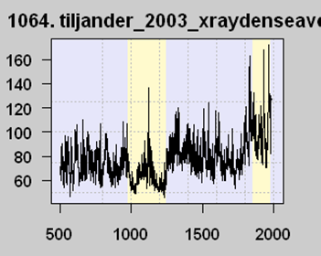
But now the interesting part.  Michael Mann, among others, used this proxy series (despite the well-know corruption) among a number of others in an attempt to model the last thousand years or so of global temperature history.   To simplify what is in fact more complicated, his models regress each proxy series like this against measured temperatures over the last 100 years or so.  But look at the last 100 years on this graph.  Measured temperatures are going up, so his regression locked onto this proxy and … flipped the sign.  In effect, it reversed the proxy.  As far as his models are concerned, this proxy is averaged in with values of the opposite sign, like this:

picture2

A number of folks, particularly Steve McIntyre, have called Mann on this, saying that he can’t flip the proxy upside down.  Mann’s response is that the regression doesn’t care about the sign, and that its all in the math.

Hopefully, after our background exposition, you see the problem.  Mann started with a theory that more organic material in lake sediments (as shown by lower x-ray densities) correlated with higher temperatures.  But his regression showed the opposite relationship — and he just accepted this, presumably because it yielded the hockey stick shape he wanted.  But there is absolutely no physical theory as to why our historic understanding of organic matter deposition in lakes should be reversed, and Mann has not even bothered to provide one.  In fact, he says he doesn’t even need to.

This mistake (fraud?) is even more egregious because it is clear that the jump in x-ray values in recent years is due to a spurious signal and corruption of the data.  Mann’s algorithm is locking into meaningless noise, and converting it into a “signal” that there is a hockey stick shape to the proxy data.

As McIntyre concludes:

In Mann et al 2008, there is a truly remarkable example of opportunistic after-the-fact sign selection, which, in addition, beautifully illustrates the concept of spurious regression, a concept that seems to baffle signal mining paleoclimatologists.

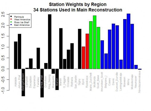
Postscript: If you want an even more absurd example of this data-mining phenomenon, look no further than Steig’s study of Antarctic temperatures.   In the case of proxies, it is possible (though unlikely) that we might really reverse our understanding of how the proxy works based on the regression results. But in Steig, they were taking individual temperature station locations and creating a relationship between them to a synthesized continental temperature number.  Steig used regression techniques to weight various thermometers in rolling up the continental measure.  But five of the weights were negative!!

bar-plot-station-weights

As I wrote then,

Do you see the problem?  Five stations actually have negative weights!  Basically, this means that in rolling up these stations, these five thermometers were used upside down!  Increases in these temperatures in these stations cause the reconstructed continental average to decrease, and vice versa.  Of course, this makes zero sense, and is a great example of scientists wallowing in the numbers and forgetting they are supposed to have a physical reality.  Michael Mann has been quoted as saying the multi-variable regression analysis doesn’t care as to the orientation (positive or negative) of the correlation.  This is literally true, but what he forgets is that while the math may not care, Nature does.

Some Common Sense on Treemometers

I have written a lot about historic temperature proxies based on tree rings, but it all boils down to “trees make poor thermometers.”  There are just too many things, other than temperature, that can affect annual tree growth.  Anthony Watts has a brief article from one of his commenter that discusses some of these issues in a real-life way.  This in particular struck me as a strong dose of common sense:

The bristlecone records seemed a lousy proxy, because at the altitude where they grow it is below freezing nearly every night, and daytime temperatures are only above freezing for something like 10% of the year. They live on the borderline of existence, for trees, because trees go dormant when water freezes. (As soon as it drops below freezing the sap stops dripping into the sugar maple buckets.) Therefore the bristlecone pines were dormant 90% of all days and 99% of all nights, in a sense failing to collect temperature data all that time, yet they were supposedly a very important proxy for the entire planet. To that I just muttered “bunkum.”

He has more on Briffa’s increasingly famous single hockey stick tree.

More Hockey Stick Hyjinx

Update: Keith Briffa responds to the issues discussed below here.

Sorry I am a bit late with the latest hockey stick controversy, but I actually had some work at my real job.

At this point, spending much time on the effort to discredit variations of the hockey stick analysis is a bit like spending time debunking phlogiston as the key element of combustion.  But the media still seems to treat these analyses with respect, so I guess the effort is necessary.

Quick background:  For decades the consensus view was that earth was very warm during the middle ages, got cold around the 17th century, and has been steadily warming since, to a level today probably a bit short of where we were in the Middle Ages.  This was all flipped on its head by Michael Mann, who used tree ring studies to “prove” that the Medieval warm period, despite anecdotal evidence in the historic record (e.g. the name of Greenland) never existed, and that temperatures over the last 1000 years have been remarkably stable, shooting up only in the last 50 years to 1998 which he said was likely the hottest year of the last 1000 years.  This is called the hockey stick analysis, for the shape of the curve.

Since he published the study, a number of folks, most prominently Steve McIntyre, have found flaws in the analysis.  He claimed Mann used statistical techniques that would create a hockey stick from even white noise.  Further, Mann’s methodology took numerous individual “proxies” for temperatures, only a few of which had a hockey stick shape, and averaged them in a way to emphasize the data with the hockey stick.  Further, Mann has been accused of cherry-picking — leaving out proxy studies that don’t support his conclusion.  Another problem emerged as it became clear that recent updates to his proxies were showing declining temperatures, what is called “divergence.”  This did not mean that the world was not warming, but did mean that trees may not be very good thermometers.  Climate scientists like Mann and Keith Briffa scrambled for ways to hide the divergence problem, and even truncated data when necessary.  More hereMann has even flipped the physical relationship between a proxy and temperature upside down to get the result he wanted.

Since then, the climate community has tried to make itself feel better about this analysis by doing it multiple times, including some new proxies and new types of proxies (e.g. sediments vs. tree rings).  But if one looks at the studies, one is struck by the fact that its the same 10 guys over and over, either doing new versions of these studies or reviewing their buddies studies.  Scrutiny from outside of this tiny hockey stick society is not welcome.  Any posts critical of their work are scrubbed from the comment sections of RealClimate.com (in contrast to the rich discussions that occur at McIntyre’s site or even this one) — a site has even been set up independently to archive comments deleted from Real Climate.  This is a constant theme in climate.  Check this policy out — when one side of the scientific debate allows open discussion by all comers, and the other side censors all dissent, which do you trust?

Anyway, all these studies have shared a couple of traits in common:

  • They have statistical methodologies to emphasize the hockey stick
  • They cherry pick data that will support their hypothesis
  • They refuse to archive data or make it available for replication

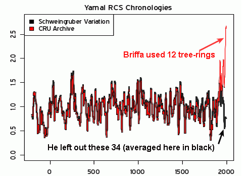
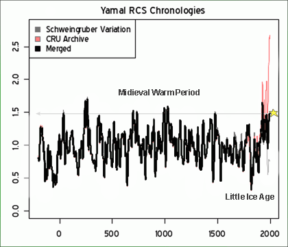
The some extent, the recent to-do about Briffa and the Yamal data set have all the same elements.  But this one appears to have a new one — not only are the data sets cherry-picked, but there is growing evidence that the data within a data set has been cherry picked.

Yamal is important for the following reason – remember what I said above about just a few data sets driving the whole hockey stick.  These couple of data sets are the crack cocaine to which all these scientists are addicted.  They are the active ingredient.  The various hockey stick studies may vary in their choice of proxy sets, but they all include a core of the same two or three that they know with confidence will drive the result they want, as long as they are careful not to water them down with too many other proxies.

Here is McIntyre’s original post.   For some reason, the data set Briffa uses falls off to ridiculously few samples in recent years (exactly when you would expect more).  Not coincidentally, the hockey stick appears exactly as the number of data points falls towards 10 and then 5 (from 30-40).  If you want a longer, but more layman’s view, Bishop Hill blog has summarized the whole storyUpdateMore here, with lots of the links I didn’t have time this morning to find.

Postscript: When backed against the wall with no response, the Real Climate community’s ultimate response to issues like this is “Well, it doesn’t matter.”  Expect this soon.

Update: Here are the two key charts, as annotated by JoNova:

rcs_chronologies1v2

And it “matters”

yamal-mcintyre-fig2

More Proxy Hijinx

Steve McIntyre digs into more proxy hijinx from the usual suspects.  This is a pretty good summary of what he tends to find, time and again in these studies:

The problem with these sorts of studies is that no class of proxy (tree ring, ice core isotopes) is unambiguously correlated to temperature and, over and over again, authors pick proxies that confirm their bias and discard proxies that do not. This problem is exacerbated by author pre-knowledge of what individual proxies look like, leading to biased selection of certain proxies over and over again into these sorts of studies.

The temperature proxy world seems to have developed into a mono-culture, with the same 10 guys creating new studies, doing peer review, and leading IPCC sub-groups.  The most interesting issue McIntyre raises is that this new study again uses proxy’s “upside down.”  I explained this issue more here and here, but a summary is:

Scientists are trying to reconstruct past climate variables like temperature and precipitation from proxies such as tree rings.  They begin with a relationship they believe exists based on a physical understanding of a particular system – ie, for tree rings, trees grow faster when its warm so tree rings are wider in warm years.  But as they manipulate the data over and over in their computers, they start to lose touch with this physical reality.

…. in one temperature reconstruction, scientists have changed the relationship opportunistically between the proxy and temperature, reversing their physical understanding of the process and how similar proxies are handled in the same study, all in order to get the result they want to get.

So Why Bother?

I just watched Peter Sinclair’s petty little video on Anthony Watt’s effort to survey and provide some level of quality control on the nation’s surface temperature network.  Having participated in the survey, I was going to do a rebuttal video from my own experience, but I just don’t have the time, but I want to offer a couple of quick thoughts.

  • Will we ever see an alarmist be able to address any skeptics critique of AGW science without resorting to ad hominem attacks?  I guess the whole “oil industry funding” thing is a base requirement for any alarmist article, but this guy really gets extra credit for the tobacco industry comparison.  Seriously, do you guys really think this addresses the issue?
  • I am fairly sure that Mr. Watt would not deny that the world has warmed over the last 100 years, though he might argue that warming has been exaggerated somewhat.  Certainly satellites are immune to the biases and problems Mr. Watt’s group is identifying, and they still show warming  (though less than the surface temperature networks is showing).
  • The video tries to make Watt’s volunteers sound like silly children at camp, but in fact weather measurement and data collection in this country have a long history of involvement and leadership by volunteers and amateurs.
  • The core point that really goes unaddressed is that the government, despite spending billions of dollars on AGW-related projects, is investing about zero in quality control of the single most critical data set to the current public policy decisions.   Many of the sites are absolutely inexcusable, EVEN against the old goals of reporting weather rather than measuring climate change.  I surveyed the Tucson site – it is a joke.
  • Mr. Sinclair argues that the absolute value of the temperatures does not matter as much as their changes over time.  Fine, I would agree.  But again, he demonstrates his ignorance.  This is an issue Anthony and most of his readers discuss all the time.  When, for example, we talk about the really biased site at Tucson, it is always in the context of the fact that 100 years ago Tucson was a one horse town, and so all the urban heat biases we might find in a badly sited urban location have been introduced during the 20th century measurement period.  These growing biases show up in the measurements as increasing temperatures.  And the urban heat island effects are huge.  My son and I personally measured about 10F in the evening.  Even if this was only at Tmin, and was 0 effect at Tmax  (daily average temps are the average of Tmin and Tmax) then this would still introduce a bias of 5F today that was surely close to zero a hundred years ago.
  • Mr. Sinclair’s knowledge about these issues is less than one of our readers might have had 3 years ago.  He says we should be satisfied with the data quality because the government promises that it has adjusted for these biases.  But these very adjustments, and the inadequacy of the process, is one reason for Mr. Watt’s efforts.  If Mr. Sinclair had bothered to educate himself, he would know that many folks have criticized these adjustments because they are done blind, without any reference to actual station quality or details, by statistical processes.  But without the knowledge of which stations have better installations, the statistical processes tend to spread the bias around like peanut butter, rather than really correct for it, as demonstrated here for Tucson and the Grand Canyon (both of these stations I have personally visited).
  • The other issue one runs into in trying to correct for a bad site through adjustments is the signal to noise problem.  The world global warming signal over the last 100 years has been no more than 1 degree F.  If urban heat biases are introducing a 5,8, or 10 degree bias, then the noise, and thus the correction factor, is 5-10 times larger than the signal.   In practical terms, this means a 10-20% error in the correction factor can completely overwhelm the signal one is trying to detect.  And since most of the correction factors are not much better than educated guesses, their errors are certainly higher than this.
  • Overall Mr. Sinclair’s point seems to be that the quality of the stations does not matter.  I find that incredible, and best illustrated with an example.  The government makes decisions about the economy and interest rates and taxes and hundreds of other programs based on detailed economic data.  Let’s say that instead of sampling all over Arizona, they just sampled in one location, say Paradise Valley zip code 85253.  Paradise Valley happens to be (I think) the wealthiest zip code in the state.  So, if by sampling only in Paradise Valley, the government decides that everyone is fine and no one needs any government aid, would Mr. Sinclair be happy?  Would this be “good enough?”  Or would we demand an investment in a better data gathering network that was not biased towards certain demographics to make better public policy decisions involving hundreds of billions of dollars?

GCCI #5: The Dog That Didn’t Bark

The GCCI is mainly focused on creating a variety of future apocalyptic narratives.  However, it was interesting none-the-less for what was missing:  No hockey stick, and no Co2/temperature 600,000 year ice core chart.  Have we finally buried these chestnuts, or were they thought unnecessary as the report really expends no effort defending the existence of warming.

Forgetting About Physical Reality

Sometimes in modeling and data analysis one can get so deep in the math that one forgets there is a physical reality those numbers are supposed to represent.  This is a common theme on this site, and a good example was here.

Jeff Id, writing at Watts Up With That, brings us another example from Steig’s study on Antarctic temperature changes.  In this study, one step Steig takes is to reconstruct older, pre-satellite continental temperature  averages from station data at a few discrete stations.  To do so, he uses more recent data to create weighting factors for the individual stations.  In some sense, this is basically regression analysis, to see what combination of weighting factors times station data since 1982 seems to be fit with continental averages from the satellite.

Here are the weighting factors the study came up with:

bar-plot-station-weights

Do you see the problem?  Five stations actually have negative weights!  Basically, this means that in rolling up these stations, these five thermometers were used upside down!  Increases in these temperatures in these stations cause the reconstructed continental average to decrease, and vice versa.  Of course, this makes zero sense, and is a great example of scientists wallowing in the numbers and forgetting they are supposed to have a physical reality.  Michael Mann has been quoted as saying the multi-variable regression analysis doesn’t care as to the orientation (positive or negative) of the correlation.  This is literally true, but what he forgets is that while the math may not care, Nature does.

For those who don’t follow, let me give you an example.  Let’s say we have market prices in a number of cities for a certain product, and we want to come up with an average.  To do so, we will have to weight the various local prices based on sizes of the city or perhaps populations or whatever.  But the one thing we can almost certainly predict is that none of the individual city weights will be negative.  We won’t, for example, ever find that the average western price of a product goes up because one component of the average, say the price in Portland, goes down.  This flies in the face of our understanding of how an arithmetic average should work.

It may happen that in a certain time periods, the price in Portland goes down in the same month as the Western average went up, but the decline in price in Portland did not drive the Western average up — in fact, its decline had to have actually limited the growth of the Western average below what it would have been had Portland also increased.   Someone looking at that one month and not understanding the underlying process might draw the conclusion that prices in Portland were related to the Western average price by a negative coefficient, but that conclusion would be wrong.

The Id post goes on to list a number of other failings of the Steig study on Antarctica, as does this post.  Years ago I wrote an article arguing that while the GISS and other bodies claim they have a statistical method for eliminating individual biases of measurement stations in their global averages, it appeared to me that all they were doing was spreading the warming bias around a larger geographic area like peanut butter.  Steig’ study appears to do the same thing, spreading the warming from the Antarctic Peninsula across the whole continent, in part based on its choice to use just three PC’s, a number that is both oddly small and coincidentally exactly the choice required to get the maximum warming value from their methodology.

Numbers Divorced from Reality

This article on Climate Audit really gets at an issue that bothers many skeptics about the state of climate science:  the profession seems to spend so much time manipulating numbers in models and computer systems that they start to forget that those numbers are supposed to have physical meaning.

I discussed the phenomenon once before.  Scientists are trying to reconstruct past climate variables like temperature and precipitation from proxies such as tree rings.  They begin with a relationship they believe exists based on an understanding of a particular system – ie, for tree rings, trees grow faster when its warm so tree rings are wider in warm years.  But as they manipulate the data over and over in their computers, they start to lose touch with this physical reality.

In this particular example, Steve McIntyre shows how, in one temperature reconstruction, scientists have changed the relationship opportunistically between the proxy and temperature, reversing their physical understanding of the process and how similar proxies are handled in the same study, all in order to get the result they want to get.

McIntyre’s discussion may be too arcane for some, so let me give you an example.  As a graduate student, I have been tasked with proving that people are getting taller over time and estimating by how much.  As it turns out, I don’t have access to good historic height data, but by a fluke I inherited a hundred years of sales records from about 10 different shoe companies.  After talking to some medical experts, I gain some confidence that shoe size is positively correlated to height.  I therefore start collating my 10 series of shoe sales data, pursuing the original theory that the average size of the shoe sold should correlate to the average height of the target population.

It turns out that for four of my data sets, I find a nice pattern of steadily rising shoe sizes over time, reflecting my intuition that people’s height and shoe size should be increasing over time.  In three of the data sets I find the results to be equivical — there is no long-term trend in the sizes of shoes sold and the average size jumps around a lot.  In the final three data sets, there is actually a fairly clear negative trend – shoe sizes are decreasing over time.

So what would you say if I did the following:

  • Kept the four positive data sets and used them as-is
  • Threw out the three equivocal data sets
  • Kept the three negative data sets, but inverted them
  • Built a model for historic human heights based on seven data sets – four with positive coefficients between shoe size and height and three with negative coefficients.

My correlation coefficients are going to be really good, in part because I have flipped some of the data sets and in part I have thrown out the ones that don’t fit initial bias as to what the answer should be.  Have I done good science?  Would you trust my output?  No?

Well what I describe is identical to how many of the historical temperature reconstruction studies have been executed  (well, not quite — I have left out a number of other mistakes like smoothing before coefficients are derived and using de-trended data).

Mann once wrote that multivariate regression methods don’t care about the orientation of the proxy. This is strictly true – the math does not care. But people who recognize that there is an underlying physical reality that makes a proxy a proxy do care.

It makes no sense to physically change the sign of the relationship of our final three shoe databases.  There is no anatomical theory that would predict declining shoe sizes with increasing heights.  But this seems to happen all the time in climate research.  Financial modellers who try this go bankrupt.  Climate modellers who try this to reinforce an alarmist conclusion get more funding.  Go figure.

Seriously?

In study 1, a certain historic data set is presented.  The data set shows an underlying variation around a fairly strong trend line.  The trend line is removed, for a variety of reasons, and the data set is presented normalized or de-trended.

In study 2, researches take the normalized, de-trended data and conclude … wait for it … that there is no underlying trend in the natural process being studied.  Am I really understanding this correctly?  I think so:

The briefest examination of the Scotland speleothem shows that the version used in Trouet et al had been previously adjusted through detrending from the MWP [Medievil Warm Period] to the present. In the original article (Proctor et al 2000), this is attributed to particularities of the individual stalagmite, but, since only one stalagmite is presented, I don’t see how one can place any confidence on this conclusion. And, if you need to remove the trend from the MWP to the present from your proxy, then I don’t see how you can use this proxy to draw to conclusions on relative MWP-modern levels.

Hope and change, climate science version.

Postscript: It is certainly possible that the underlying data requires an adjustment, but let’s talk about why the adjustment used is not correct.  The scientists have a hypothesis that they can look at the growth of stalagmites in certain caves and correlate the annual growth rate with climate conditions.

Now, I could certainly imagine  (I don’t know if this is true, but work with me here) that there is some science that the volume of material deposited on the stalagmite is what varies in different climate conditions.  Since the stalagmite grows, a certain volume of material on a smaller stalagmite would form a thicker layer than the same volume on a larger stalagmite, since the larger body has a larger surface area.

One might therefore posit that the widths could be corrected back to the volume of the material deposited based on the width and height of the stalagmite at the time (if these assumptions are close to the mark, it would be a linear, first order correction since surface area in a cone varies linearly with height and radius).  There of course might be other complicating factors beyond this simple model — for example, one might argue that the deposition rate might itself change with surface area and contact time.

Anyway, this would argue for a correction factor based on geometry and the physics / chemistry of the process.  This does NOT appear to be what the authors did, as per their own description:

This band width was signal was normalized and the trend removed by fitting an order 2 polynomial trend line to the band width data.

That can’t be right.  If we don’t understand the physics well enough to know how, all things being equal, band widths will vary by size of the stalagmite, then we don’t understand the physics well enough to use it confidently as a climate proxy.

Steve McIntyre on the Hockey Stick

I meant to post this a while back, and most of my readers will have already seen this, but in case you missed it, here is Steve McIntyre’s most recent presentation on a variety of temperature reconstruction issues, in particular Mann’s various new attempts at resuscitating the hockey stick.  While sometimes his web site Climate Audit is hard for laymen and non-statisticians to follow, this presentation is pretty accessible.

Worth Your Time

I really like to write a bit more about such articles, but I just don’t have the time right now.  So I will simply recommend you read this guest post at WUWT on Steig’s 2009 Antarctica temperature study.  The traditional view has been that the Antarctic Peninsula (about 5% of the continent) has been warming a lot while the rest of the continent has been cooling.  Steig got a lot of press by coming up with the result that almost all of Antarctica is warming.

But the article at WUWT argues that Steig gets to this conclusion only by reducing all of Antarctic temperatures to three measurement points.  This process smears the warming of the peninsula across a broader swath of the continent.  If you can get through the post, you will really learn a lot about the flaws in this kind of study.

I have sympathy for scientists who are working in a low signal to noise environment.   Scientists are trying to tease 50 years of temperature history across a huge continent from only a handful of measurement points that are full of holes in the data.  A charitable person would look at this article and say they just went too far, teasing out spurious results rather than real signal out of the data.  A more cynical person might argue that this is a study where, at every turn, the authors made every single methodological choice coincidentally in the one possible way that would maximize their reported temperature trend.

By the way, I have seen Steig written up all over, but it is interesting that I never saw this:  Even using Steig’s methodology, the temperature trend since 1980 has been negative.  So whatever warming trend they found ended almost 30 years ago.    Here is the table from the WUWT article, showing the Steign original results and several cuts and recalculating their data using improved methods.

Reconstruction

1957 to 2006 trend

1957 to 1979 trend (pre-AWS)

1980 to 2006 trend (AWS era)

Steig 3 PC

+0.14 deg C./decade

+0.17 deg C./decade

-0.06 deg C./decade

New 7 PC

+0.11 deg C./decade

+0.25 deg C./decade

-0.20 deg C./decade

New 7 PC weighted

+0.09 deg C./decade

+0.22 deg C./decade

-0.20 deg C./decade

New 7 PC wgtd imputed cells

+0.08 deg C./decade

+0.22 deg C./decade

-0.21 deg C./decade

Here, by the way, is an excerpt from Steig’s abstract in Nature:

Here we show that significant warming extends well beyond the Antarctic Peninsula to cover most of West Antarctica, an area of warming much larger than previously reported. West Antarctic warming exceeds 0.1 °C per decade over the past 50 years, and is strongest in winter and spring.

Hmm, no mention that this trend reversed half way through the period.  A bit disengenuous, no?  Its almost as if there is a way they wanted the analysis to come out.

The First Rule of Regression Analysis

Here is the first thing I was ever taught about regression analysis — never, ever use multi-variable regression analysis to go on a fishing expedition.  In other words, never throw in a bunch of random variables and see what turns out to have the strongest historical relationship.  Because the odds are that if you don’t understand the relationship between the variables and why you got the answer that you did, it is very likely a spurious result.

The purpose of a regression analysis is to confirm and quantify a relationship that you have a theoretical basis for believing to exist.  For example, I might think that home ownership rates might drop as interest rates rose, and vice versa, because interest rate increases effectively increase the cost of a house, and therefore should reduce the demand.  This is a perfectly valid proposition to test.  What would not be valid is to throw interest rates, population growth, regulatory levels, skirt lengths,  superbowl winners, and yogurt prices together into a regression with housing prices and see what pops up as having a correlation.   Another red flag would be, had we run our original regression between home ownership and interest rates and found the opposite result than we expected, with home ownership rising with interest rates, we need to be very very suspicious of the correlation.  If we don’t have a good theory to explain it, we should treat the result as spurious, likely the result of mutual correlation of the two variables to a third variable, or the result of time lags we have not considered correctly, etc.

Makes sense?  Well, then, what do we make of this:  Michael Mann builds temperature reconstructions from proxies.  An example is tree rings.  The theory is that warmer temperatures lead to wider tree rings, so one can correlate tree ring growth to temperature.  The same is true for a number of other proxies, such as sediment deposits.

In the particular case of the Tiljander sediments, Steve McIntyre observed that Mann had included the data upside down – meaning he had essentially reversed the sign of the proxy data.  This would be roughly equivalent to our running our interest rate – home ownership regression but plugging the changes in home ownership with the wrong sign (ie decreases shown as increases and vice versa).

You can see that the data was used upside down by comparing Mann’s own graph with the orientation of the original article, as we did last year. In the case of the Tiljander proxies, Tiljander asserted that “a definite sign could be a priori reasoned on physical grounds” – the only problem is that their sign was opposite to the one used by Mann. Mann says that multivariate regression methods don’t care about the orientation of the proxy.

The world is full of statements that are strictly true and totally wrong at the same time.  Mann’s statement in bold is such a case.  This is strictly true – the regression does not care if you get the sign right, it will still get a correlation.  But it is totally insane, because this implies that the correlation it is getting is exactly the opposite of what your physics told you to expect.  It’s like getting a positive correlation between interest rates and home ownership.  Or finding that tree rings got larger when temperatures dropped.

This is a mistake that Mann seems to make a lot — he gets buried so far down into the numbers, he forgets that they have physical meaning.  They are describing physical systems, and what they are saying in this case makes no sense.  He is essentially using a proxy that is essentially behaving exactly the opposite of what his physics tell him it should – in fact behaving exactly opposite to the whole theory of why it should be a proxy for temperature in the first place.  And this does not seem to bother him enough to toss it out.

PS-  These flawed Tiljander sediments matter.  It has been shown that the Tiljander series have an inordinate influence on Mann’s latest proxy results.  Remove them, and a couple of other flawed proxies  (and by flawed, I mean ones with manually made up data) and much of the hockey stick shape he loves so much goes away

We Eliminated Everything We Could Think Of, So It Has To Be Warming

I am still trying to get a copy of the article in Science on which this is based, but the AZ Republic writes:

Western forests that withstood wildfire, insect attacks and drought are now withering under an even greater menace.

Heat.

Rising temperatures are wiping out trees faster than the forests can replace them, killing pines, firs, hemlocks and almost every other kind of tree at almost every elevation from northern Arizona to southwestern Canada.

Writing today in the journal Science, a team of 11 researchers says global warming is almost certainly the culprit behind a sharp spike in tree deaths over the past several decades. The higher death rates, which doubled in as few as 17 years in some areas, coincide with a regional increase in temperature and appear unrelated to other outside factors.

Perhaps this question is answered somewhere in the unreported details, but my first reaction was to want to ask “Dendroclimatologists like Michael Mann reconstruct history from tree rings based on the assumption that increasing temperatures correlates linearly and positively with tree growth and therefore tree ring width.  Your study seems to indicate the correlation between tree growth and temperature is negative and probably non-linear.  Can you reconcile these claims?’    Seriously, there may be an explanation (different kinds of trees?) but after plastering the hockey stick all over the media for 10 years, no one even thinks to ask?

Normally, I just ignore the flood of such academic work  (every study nowadays has global warming in it — if these guys had just wanted to study the forest, they would have struggled for grant money, but make it about forest and global warming and boom, here’s your money).  The reasons I picked it out was because I just love the quote below — I can’t tell you how often I see this in climate science-related work:

Scientists combed more than 50 years of data that included tree counts and conditions. The sharp rise in tree mortality was apparent quickly. Researchers then eliminated possible causes for the tree deaths, such as air pollution, fire suppression or overgrowth. They concluded the most likely culprit was heat.

Again, I need to see the actual study, but this would not be the first time a climate study said “well, we investigated every cause we could think of, and none of them seemed to fit, so it must be global warming.”  It’s a weird way to conduct science, assuming Co2 and warming are the default cause for every complex natural process.  No direct causal relationship is needed with warming, all that is required is to eliminate any other possible causes.  This means that the less well we understand any complex system, the more likely we are to determine changes in the system are somehow anthropogenic.

Speaking of anthropogenic, I am fairly certain that the authors have not even considered the most likely anthropogenic cause, if the source of the forest loss is even man-made at all.  From my reading of the literature, nearby land use changes (clearing forests for agriculture, urbanization, etc) have a much greater affect on local climates and particularly moisture patterns than does a general global warming trend.  If you clear all the surrounding forest, it is likely that the piece that is left is not as healthy as it would have been in the midst of other forested land.

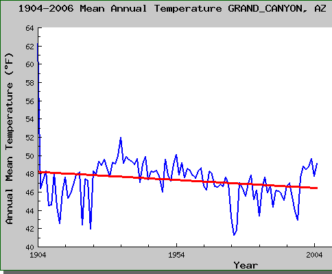
The article, probably because it is making an Arizona connection, makes a big deal about the role of a study forest near Flagstaff in the study.  But if the globe is warming, the area around Norther Arizona has not really been participating.  The nearest station to the forest is the USHCN station at the Grand Canyon, a pretty decent analog because it is nearby, rural, and forested as well.  Here is the plot of temperatures from that station:

grand_canyon_temp

Its hard to tell from the article, but my guess is that there is actually a hidden logic leap embedded.  Likely, their finding is that drought has stressed trees and reduced growth.  They then rely on other studies to say that this drought is due to global warming, so then they can get to the grant-tastic finding that global warming is hurting the forest.   But the “western drought caused mainly by anthropogenic warming” is not a well proven connection.  Warming likely has some contribution to it, but the west has been through wet-dry cycles for tens of thousands of years, and has been through much worse and longer droughts long before the Clampetts started pumping black gold from the ground.

Linear Regression Doesn’t Work if the Underlying Process is not Linear

Normally, I would have classified the basic premise of Craig Loehle's recent paper, as summarized at Climate Audit, as a blinding glimpse of the obvious.  Unfortunately, the climate science world is in desperate need of a few BGO's, so the paper is timely.  I believe his premise can be summarized as follows:

  1. Many historical temperature reconstructions, like Mann's hockey stick, use linear regressions to translate tree ring widths into past temperatures
  2. Linear regressions don't work when the underlying relationship, here between tree rings and temperature, is not linear.

The relationship between tree ring growth and temperature is almost certainly non-linear.  For example, tree ring growth does not go up forever, linearly, with temperature.  A tree that grows 3mm in a year at 80F and 4mm at 95F is almost certainly not going to grow 6mm at 125F. 

However, most any curve, over a sufficiently narrow range, can be treated as linear for the purposes of most analyses.  The question here is, given the relationship between tree ring growth and temperatures, do historical temperatures fall into such a linear region?  I think it is increasingly obvious the answer is "no," for several reasons:

  1. There is simply not very good, consistent data on the behavior of tree ring growths with temperature from folks like botanists rather than climate scientists.  There is absolutely no evidence whether we can treat ring widths as linear with temperatures over a normal range of summer temperatures.
  2. To some extent, folks like Mann (author of the hockey stick) are assuming their conclusion.  They are using tree ring analysis to try to prove the hypothesis that historic temperatures stayed in a narrow band (vs. current temperatures that are, they claim, shooting out of that band).  But to prove this, they must assume that temperatures historically remained in a narrow band that is the linear range of tree ring growth.  Essentially, they have to assume their conclusion to reach their conclusion.
  3. There is strong evidence that tree rings are not very good, linear measurements of temperature due to the divergence issue.  In short — Mann's hockey stick is only hockey stick shaped if one grafts the surface temperature record onto the tree ring history.  Using only tree ring data through the last few decades shows no hockey stick.  Tree rings are not following current rises in temperatures, and so it is likely they underestimate past rises in temperature.  Much more here.

  4. Loehle's pursues several hypotheticals, and demonstrates that a non-linear relationship of tree rings to temperature would explain the divergence problem and would make the hockey stick a completely incorrect reconstruction.

NOAA Adjustments

Anthony Watts has an interesting blink comparisonbetween the current version of history from the GISS and their version of history in 1999.  It is amazing that all of the manual adjustments they add to the raw data constantly have the effect of increasing historical warming.  By continuing to adjust recent temperatures up, and older temperatures down, they are implying that current measurement points have a cooling bias vs. several decades ago.  REALLY?  This makes absolutely no sense given what we now know via Anthony Watt’s efforts to document station installation details at surfacestations.org.

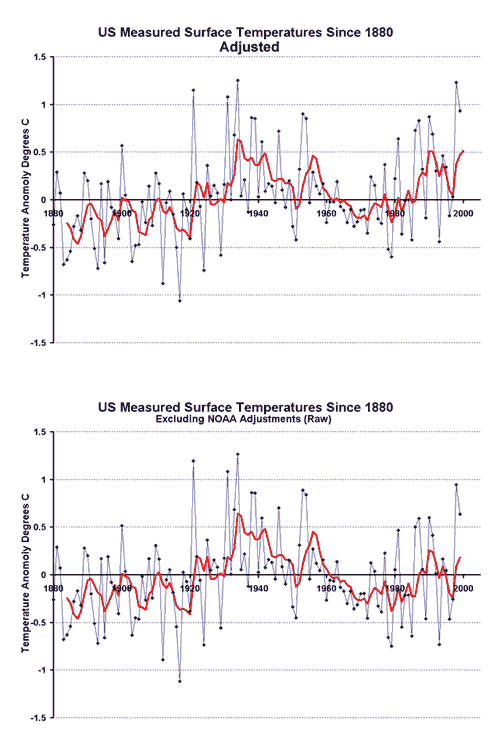
I created a blink comparison a while back that was related but slightly different.  I created a blink comparison to show the effect of NOAA manual adjustments to the raw temperature data.

adjustments

My point was not that all these adjustments were unnecessary (the time of observation adjustment is required, though I have always felt it to be exaggerated).  But all of the adjustments are upwards, even those for station quality.  The net effect is that there is no global warming signal in the US, at least in the raw data.  The global warming signal emerges entirely from the manual adjustments.  Which causes one to wonder as to the signal to noise ratio here.  And increases the urgency to get more scrutiny on these adjustments.

It only goes through 2000, because I only had the adjustment numbers through 2000.  I will see if I can update this.

Lipstick on a Pig

Apparently, Michael Mann is yet again attempting a repackaging of his hockey stick work.  The question is, has he re-worked his methodologies to overcome the many statistical issues third parties have had with his work, or is this more like AirTran changing its name from ValuJet to escape association in people’s mind with its 1996 plane crash?

Well, Steve McIntyre is on the case, and from first glance, the new Mann work seems to be the same old mish-mash of cherry-picked proxies, bizarre statistical methods, and manual tweaking of key proxies to make them look the way Mann wants them to look.  One thing I had never done was look at all the component proxies of the temperature reconstructions all in one place.  At the link above, Steve has all the longer ones in a animated GIF.  It is really striking how a) almost none of them have a hockey stick shape and b) even the few that do have HS shapes typically show the warming trend beginning in 1800, not in the late 19th century CO2 period. 

If you would like to eyeball all 1209 of the proxies Mann begins with (before he starts cherry picking), they are linked here.  I really encourage you to click through to one of the five animations, just to get  a feel for it.  As someone who has done a lot of data analysis, it is just staggering that he can get a hockey stick out of these and claim that it is in some way statistically significant.  It is roughly equivalent to watching every one of your baseball team’s games, seeing them lose each one, and then being told that they have the best record in the league.  It makes no sense.

The cherry-picking is just staggering, though you have to read the McIntyre articles as a sort of 2-3 year serial to really get the feel of it.  However, this post gives one a feel of how Mann puts a thin statistical-sounding veneer to cover his cherry-picking, but at the end of the day, he has basically invented a process that takes about a thousand proxy series and kicks out all but the 484 that will generate a hockey stick.

Update:  William Briggs finds other problems with Mann’s new analysis:

The various black lines are the actual data! The red-line is a 10-year running mean smoother! I will call the black data the real data, and I will call the smoothed data the fictional data. Mann used a “low pass filter” different than the running mean to produce his fictional data, but a smoother is a smoother and what I’m about to say changes not one whit depending on what smoother you use.

Now I’m going to tell you the great truth of time series analysis. Ready? Unless the data is measured with error, you never, ever, for no reason, under no threat, SMOOTH the series! And if for some bizarre reason you do smooth it, you absolutely on pain of death do NOT use the smoothed series as input for other analyses! If the data is measured with error, you might attempt to model it (which means smooth it) in an attempt to estimate the measurement error, but even in these rare cases you have to have an outside (the learned word is “exogenous”) estimate of that error, that is, one not based on your current data.

If, in a moment of insanity, you do smooth time series data and you do use it as input to other analyses, you dramatically increase the probability of fooling yourself! This is because smoothing induces spurious signals—signals that look real to other analytical methods. No matter what you will be too certain of your final results! Mann et al. first dramatically smoothed their series, then analyzed them separately. Regardless of whether their thesis is true—whether there really is a dramatic increase in temperature lately—it is guaranteed that they are now too certain of their conclusion.

and further:

The corollary to this truth is the data in a time series analysis is the data. This tautology is there to make you think. The data is the data! The data is not some model of it. The real, actual data is the real, actual data. There is no secret, hidden “underlying process” that you can tease out with some statistical method, and which will show you the “genuine data”. We already know the data and there it is. We do not smooth it to tell us what it “really is” because we already know what it “really is.”

Update:  I presume it is obvious, but the commenter "mcIntyre" has no relation that I know of to the "mcintyre" quoted and referred to in the post.  As a reminder of my comment policy, 1) I don’t ban or delete anything other than outright spam and 2) I strongly encourage everyone who agrees with me to remain measured and civil in your tone — everyone else is welcome to make as big of an ass out of him or herself as they wish.

By the way, to the commenter named "mcintyre,"  I have never ever seen the other McIntyre (quoted in this post) argue that CO2 does not act as a greenhouse gas.  He spends most of his time arguing that the statistical methods used in certain historic temperature reconstructions (e.g. Mann’s hockey stick but also 20th century instrument rollup’s like the GISS global temperature anamoly) are flawed.  I have read his blog for 3 years now and can honestly say I don’t know what his position on the magnitude of future anthropogenic warming is.  Mr. McIntyre is apparenlty not alone — Ian Jolliffe holds the opinion that the reputation of climate science is being hurt by the statistical sloppiness in certain corners of dendro-climatology.

Global Warming “Fingerprint”

Many climate scientists say they see a "fingerprint" in recent temperature increases that they claim is distinctive and makes current temperature increases different from past "natural" temperature increases. 

So, to see if we are all as smart as the climate scientists, here are two 51-year periods from the 20th century global temperature record as provided by the Hadley CRUT3.  Both are scaled the same (each line on the y-axis is 0.2C, each x-axis division is 5 years) — in fact, both are clips from the exact same image.  So, which is the anthropogenic warming and which is the natural? 

  Periodb       Perioda_3

One clip is from 1895 to 1946 (the"natural" period) and one is from 1957 to present  (the supposedly anthropogenic period). 

If you have stared at these charts long enough, the el Nino year of 1998 has a distinctive shape that I recognize, but otherwise these graphs look surprisingly similar.  If you are still not sure, you can find out which is which here.

Backcasting with Computer Climate Models

I found the chart below in the chapter Global Climate Change of the NOAA/NASA CCSP climate change report. (I discuss this report more here). I thought it was illustrative of some interesting issues:
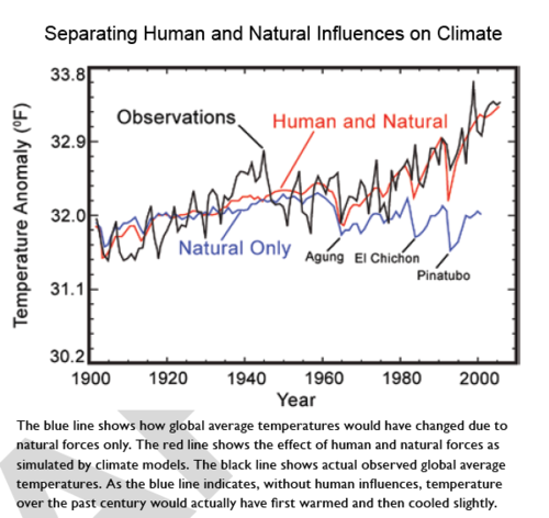
Temp

The Perfect Backcast

What they are doing is what I call "backcasting," that is, taking a predictive model and running it backwards to see how well it preforms against historical data.  This is a perfectly normal thing to do.

And wow, what a fit.  I don’t have the data to do any statistical tests, but just by eye, the red model output line does an amazing job at predicting history.  I have done a lot of modeling and forecasting in my life.  However, I have never, ever backcast any model and gotten results this good.  I mean it is absolutely amazing.

Of course, one can come up with many models that backcast perfectly but have zero predictive power

A recent item of this ilk maintains that the results of the last game played at home by the NFL’s Washington Redskins (a football team based in the national capital, Washington, D.C.) before the U.S. presidential elections has accurately foretold the winner of the last fifteen of those political contests, going back to 1944. If the Redskins win their last home game before the election, the party that occupies the White House continues to hold it; if the Redskins lose that last home game, the challenging party’s candidate unseats the incumbent president. While we don’t presume there is anything more than a random correlation between these factors, it is the case that the pattern held true even longer than claimed, stretching back over seventeen presidential elections since 1936.

And in fact, our confidence in the climate models based on their near-perfect back-casting should be tempered by the fact that when the models first were run backwards, they were terrible at predicting history.  Only a sustained effort to tweak and adjust and plug them has resulted in this tight fit  (we will return to the subject of plugging in a minute).

In fact, it is fairly easy to demonstrate that the models are far better at predicting history than they are at predicting the future.  Like the Washington Redskins algorithm, which failed in 2004 after backcasting so well, climate models have done a terrible job in predicting the first 10-20 years of the future.  This is the reason that neither this nor any other global warming alarmist report every shows a chart grading how model forecasts have performed against actual data:  Because their record has been terrible.  After all, we have climate model forecasts data all the way back from the late 1980’s — surely 20+ years is enough to get a test of their performance.

Below is the model forecasts James Hansen, whose fingerprints are all over this report, used before Congress in 1988 (in yellow, orange, and red), with a comparison to the actual temperature record (in blue).  (source)
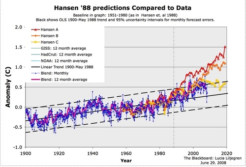
Hansenlineartrend

Here is the detail from the right side:
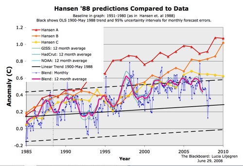
Hansencomparedrecent

You can see the forecasts began diverging from reality even as early as 1985.  By the way, don’t get too encouraged by the yellow line appearing to be fairly close — the Hansen C case in yellow was similar to the IPCC B1 case which hypothesizes strong international CO2 abatement programs which have not come about.  Based on actual CO2 production, the world is tracking, from a CO2 standpoint, between the orange and red lines.  However, temperature is no where near the predicted values.

So the climate models are perfect at predicting history, but begin diverging immediately as we move into the future.  That is probably why the IPCC resets its forecasts every 5 years, so they can hit the reset button on this divergence.  As an interesting parallel, temperature measurements of history with trees have very similar divergence issues when carried into the future.

What the Hell happened in 1955?

Looking again at the backcast chart at the top of this article, peek at the blue line.  This is what the models predict to have been the world temperature without man-made forcings.  The blue line is supposed to represent the climate absent man.  But here is the question I have been asking ever since I first started studying global warming, and no one has been able to answer:  What changed in the Earth’s climate in 1955?  Because, as you can see, climate forecasters are telling us the world would have reversed a strong natural warming trend and started cooling substantially in 1955 if it had not been for anthropogenic effects.

This has always been an issue with man-made global warming theory.  Climate scientists admit the world warmed from 1800 through 1955, and that most of this warming was natural.  But somehow, this natural force driving warming switched off, conveniently in the exact same year when anthropogenic effects supposedly took hold.  A skeptical mind might ask why current warming is not just the same natural trend as warming up to 1955, particularly since no one can say with any confidence why the world warmed up to 1955 and why this warming switched off and reversed after that.

Well, lets see if we can figure it out.  The sun, despite constant efforts by alarmists to portray it is climactically meaningless, is a pretty powerful force.  Did the sun change in 1955? (click to enlarge)
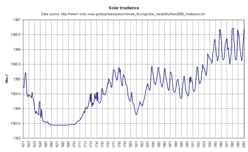
Irradiance

Well, it does not look like the sun turned off.  In fact, it appears that just the opposite was happening — the sun hit a peak around 1955 and has remained at this elevated level throughout the current supposedly anthropogenic period.

OK, well maybe it was the Pacific Decadal Oscillation?  The PDO goes through warm and cold phases, and its shifts can have large effects on temperatures in the Northern Hemisphere.
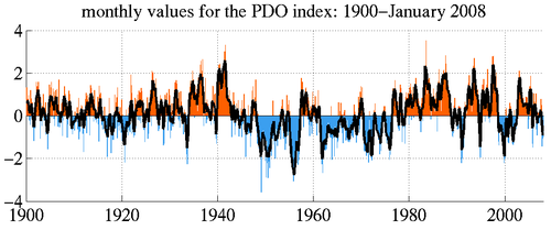
Pdo_monthly

Hmm, doesn’t seem to be the PDO.  The PDO turned downwards 10 years before 1955.  And besides, if the line turned down in 1955 due to the PDO, it should have turned back up in the 1980’s as the PDO went to its warm phase again. 

So what is it that happened in 1955.  I can tell you:  Nothing. 

Let me digress for a minute, and explain an ugly modeling and forecasting concept called a "plug".  It is not unusual that when one is building a model based on certain inputs (say, a financial model built from interest rates and housing starts or whatever) that the net result, while seemingly logical, does not get to what one thinks the model should be saying.  While few will ever admit it, I have been inside the modeling sausage factory for enough years that it is common to add plug figures to force a model to reach an answer one thinks it should be reaching — this is particularly common after back-casting a model.

I can’t prove it, any more than this report can prove the statement that man is responsible for most of the world’s warming in the last 50 years.  But I am certain in my heart that the blue line in the backcasting chart is a plug.  As I mentioned earlier, modelers had terrible success at first matching history with their forecasting models.  In particular, because their models showed such high sensitivity of temperature to CO2 (this sensitivity has to be high to get catastrophic forecasts) they greatly over-predicted history. 

Here is an example.  The graph below shows the relationship between CO2 and temperature for a number of sensitivity levels  (the shape of the curve was based on the IPCC formula and the process for creating this graph was described here).
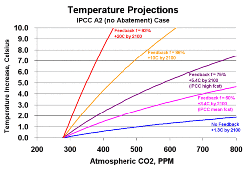
Agwforecast1

The purple lines represent the IPCC forecasts from the fourth assessment, and when converted to Fahrenheit from Celsius approximately match the forecasts on page 28 of this report.  The red and orange lines represent more drastic forecasts that have received serious consideration.  This graph is itself a simple model, and we can actually backcast with it as well, looking at what these forecasts imply for temperature over the last 100-150 years, when CO2 has increased from 270 ppm to about 385 ppm.
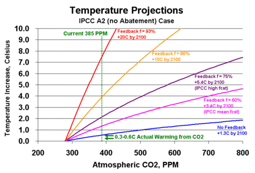
Agwforecast2

The forecasts all begin at zero at the pre-industrial number of 270ppm.  The green dotted line is the approximate concentration of CO2 today.  The green 0.3-0.6C arrows show the reasonable range of CO2-induced warming to date.  As one can see, the IPCC forecasts, when cast backwards, grossly overstate past warming.  For example, the IPCC high case predicts that we should have see over 2C warming due to CO2 since pre-industrial times, not 0.3 or even 0.6C

Now, the modelers worked on this problem.   One big tweak was to assign an improbably high cooling effect to sulfate aerosols.  Since a lot of these aerosols were produced in the late 20th century, this reduced their backcasts closer to actuals.  (I say improbably, because aerosols are short-lived and cover a very limited area of the globe.  If they cover, say, only 10% of the globe, then their cooling effect must be 1C in their area of effect to have even a small 0.1C global average effect).

Even after these tweaks, the backcasts were still coming out too high.  So, to make the forecasts work, they asked themselves, what would global temperatures have to have done without CO2 to make our models work?  The answer is that if the world naturally were to have cooled in the latter half of the 20th century, then that cooling could offset over-prediction of temperatures in the models and produce the historic result.  So that is what they did.  Instead of starting with natural forcings we understand, and then trying to explain the rest  (one, but only one, bit of which would be CO2), modelers start with the assumption that CO2 is driving temperatures at high sensitivities, and natural forcings are whatever they need to be to make the backcasts match history.

By the way, if you object to this portrayal, and I will admit I was not in the room to confirm that this is what the modelers were doing, you can do it very simply.  Just tell me what substantial natural driver of climate, larger in impact that the sun or the PDO, reversed itself in 1955.

A final Irony

I could go on all day making observations on this chart, but I would be surprised if many readers have slogged it this far.  So I will end with one irony.  The climate modelers are all patting themselves on the back for their backcasts matching history so well.  But the fact is that much of this historical temperature record is fraught with errors.  Just as one example, measured temperatures went through several large up and down shifts in the 40’s and 50’s solely because ships were switching how they took sea surface temperatures (engine inlet sampling tends to yield higher temperatures than bucket sampling).  Additionally, most surface temperature readings are taken in cities that have experienced rapid industrial growth, increasing urban heat biases in the measurements.  In effect, they have plugged and tweaked their way to the wrong target numbers!  Since the GISS and other measurement bodies are constantly revising past temperature numbers with new correction algorithms, it will be interesting to see if the climate models magically revise themselves and backcast perfectly to the new numbers as well.

More on “the Splice”

I have written that it is sometimes necesary to splice data gathered from different sources, say when I suggested splicing satellite temperature measurements onto surface temperature records.

When I did so, I cautioned that there can be issues with such splices.  In particular, one needs to be very, very careful not to make too much of an inflextion in the slope of the data that occurs right at the splice.  Reasonable scientific minds would wonder if that inflection point was an artifact of the changes in data source and measurement technology, rather than in the underlying phenomenon being measured.  Of course, climate sceintists are not reasonable, and so they declare catastrophic anthropogenic global warming to be settled science based on an inflection in temperature data right at a data source splice (between tree rings and thermometers).  More here.